Reverse Mode Autodifferentiation Explained

Reverse Mode Autodifferentiation Explained

This article is my attempt to explain reverse mode autodifferentiation to myself and hopefully to anyone else that finds this useful. (Link to notebook)

Why autodifferentiation?

The reason we prefer autodifferentiation over symbolic differentiation is due to its efficiency and simplicity. Instead of writing out explicit derivatives or parsing complex expressions and finding their symbolic derivatives, we can just compute a derivative at a particular value directly with the help of autodifferentiation.

Evaluation Trace

Before we can start differentiating, we need to create an evaluation trace. An evaluation trace essentially shows the order of operations in the form of a graph like the one below:

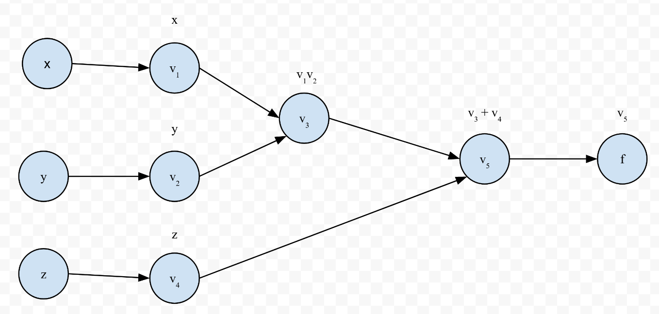
This evaluation trace represents the equation . The nodes that you see in between the output and are called intermediate variables. Now we'll look at how this evaluation trace can be used to compute a derivative.

Differentiation

This essentially boils down to using the chain rule. To compute , we do the following:

Note that since the children of , , are functions of and is a function of those children, we can apply the chain rule. The and are called adjoint variables. We'll use the evaluation trace for the example above to calculate . Since , we can calculate as follows:

So to calculate , we need to calculate . Let's try to calculate :

And now we need to compute ...but 's only child is and , so . So, now we can compute ! But what about ? Well, we know that . Initially, you might think we would try to use some fancy chain rule stuff to programatically do this, but we don't have to. We already know that if , then . This is a crucial aspect for understanding autodifferentiation: we know how to compute the derivatives of elementary functions, so we can use that to compute if is a child node of . In our example, we know , so we can use our knowledge of differentiating addition to get . If , then we would use our knowledge of differentiating subtraction to get . If , then . From a programming perspective, this means we need to (1) track which operation is being done and (2) have some way to look up how to compute the gradient of that function. If this doesn't make sense right now, don't worry, we'll write some code that reflects what is happening above. We now have all the information necessary to compute :

Also:

It bears repeating that while we are using symbols to express these derivatives here, when we program this we will be using concrete values for etc. The procedure above has returned the right answer for , since . Also notice how we computed by first computing , then , and then finally . This is why the procedure is called reverse-mode autodifferentiation.

Code

We will write a small reverse-autodifferentiation program that emulates Pytorch's interface. Namely, we want to be able to do the following:

x = Tensor(3)
y = Tensor(10)
z = x * x + x * y
z.backward()
print(x.grad) # Should print out 2 * 3 + 10 = 16
print(y.grad) # Should print out 3

Here's the code below:

def _add_grad_fn(a, b, grad):
    a.grad = grad * 1 if a.grad is None else a.grad + grad * 1
    if a.grad_fn is not None:
        a.grad_fn(*a.inputs, a.grad)
    b.grad = grad * 1 if b.grad is None else b.grad + grad * 1
    if b.grad_fn is not None:
        b.grad_fn(*b.inputs, b.grad)

def _multiply_grad_fn(a, b, grad):
    a.grad = grad * b.value if a.grad is None else a.grad + grad * b.value
    if a.grad_fn is not None:
        a.grad_fn(*a.inputs, a.grad)
    b.grad = grad * a.value if b.grad is None else b.grad + grad * a.value
    if b.grad_fn is not None:
        b.grad_fn(*b.inputs, b.grad)

class Tensor:
    def __init__(self, value, inputs=[], grad_fn=None):
        self.inputs = inputs
        self.value = value
        self.grad = None
        self.grad_fn = grad_fn

    def __add__(self, b):
        return Tensor(self.value + b.value, inputs=[self, b], grad_fn=_add_grad_fn)

    def __mul__(self, b):
        return Tensor(self.value * b.value, inputs=[self, b], grad_fn=_multiply_grad_fn)
    __rmul__ = __mul__

    # This is just to render the tensor as a string
    def __str__(self):
        return f'Tensor({self.value})'
    __repr__ = __str__
        
    def backward(self):
        if self.grad_fn is not None:
            self.grad = 1
            self.grad_fn(*self.inputs, self.grad)
        else:
            raise Exception('grad_fn is None, probably because this tensor isn\'t the result of a computation')

x = Tensor(3)
y = Tensor(10)
z = x * x + x * y
z.backward()
x.grad, y.grad

(16, 3)

Ok, so how does this relate back to what we've seen? First, let's look at the evaluation trace for :

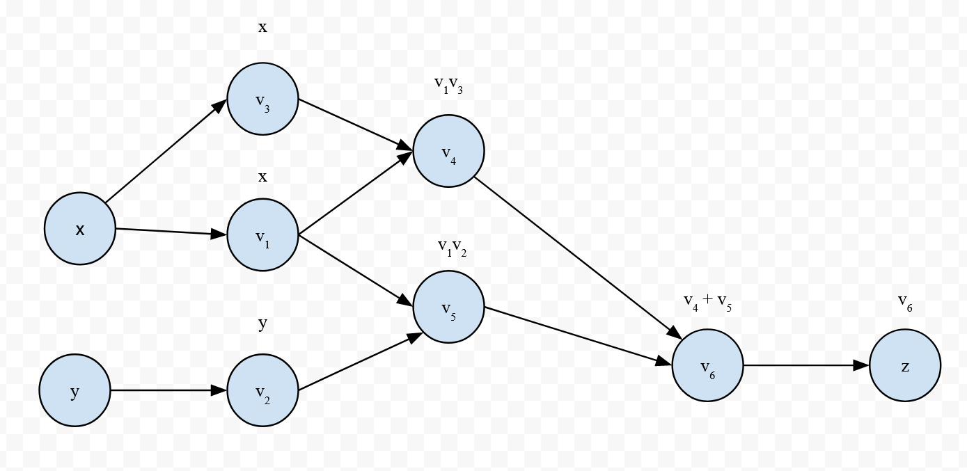
Now, we'll step through the code. The key behind this is that each tensor retains its value, a set of inputs that were used to create it (by default, none), a grad variable to track the value of its gradient, and a grad_fn variable to track a gradient function, which is used to compute the . By default, there is no gradient function, because if I create a tensor (e.g, x = Tensor(3)) with only a value, there are no derivatives we can compute (i.e, x is a constant, not a function of other variables). Furthermore, the grad variable is set to None instead of 0 to indicate that no gradient has been computed yet (as 0 could very well be the computed gradient).

Note that I also use the term "tensor" here. Normally, we would compute these derivatives with respect to a vector or matrix of values instead of just a single scalar like we did above. For simplicity's sake, I decided to keep the code to scalars, but it can be easily extended to vectors, matrices, or tensors if you wish.

Let's see what happens when we call z.backward():

def backward(self):
    if self.grad_fn is not None:
        self.grad = 1
        self.grad_fn(*self.inputs, self.grad)
    else:
        raise Exception('grad_fn is None, probably because this tensor isn\'t the result of a computation')

We first check that there is a gradient function to call. Assuming there is one, we set the gradient to one and call the gradient function of this tensor. In any computation, the last intermediate variable will always be , since if is the last intermediate variable and , then . In the evaluation trace for , . Similarly, for , . Following that, we call the current tensor's gradient function, passing in its inputs and its gradient (which is ). In the current example, this means passing in (self.grad) and (self.inputs). If you're not familiar with Python, the asterisk in *self.inputs simply splices the list into the argument list of self.grad_fn, so foo(*[1, 2]) becomes foo(1, 2). The gradient function is the core of this. Where is grad_fn assigned, you might ask? We overload the multiplication and addition operator for the Tensor class so that when we add/multiply two tensors, we get a tensor. This is where we not only set the gradient function to call, but the inputs as well:

def __add__(self, b):
    return Tensor(self.value + b.value, inputs=[self, b], grad_fn=_add_grad_fn)

def __mul__(self, b):
    return Tensor(self.value * b.value, inputs=[self, b], grad_fn=_multiply_grad_fn)
__rmul__ = __mul__

Since is equal to , it is the result of an addition, so the grad_fn variable points to the _add_grad_fn function. Let's look at it:

def _add_grad_fn(a, b, grad):
    a.grad = grad * 1 if a.grad is None else a.grad + grad * 1
    if a.grad_fn is not None:
        a.grad_fn(*a.inputs, a.grad)
    b.grad = grad * 1 if b.grad is None else b.grad + grad * 1
    if b.grad_fn is not None:
        b.grad_fn(*b.inputs, b.grad)

Again, grad is right now and a and b are and , respectively. What the gradient function does is compute and . Let's look at the computation of a.grad and what happens right after. First, we see this peculiar line:

a.grad = grad * 1 if a.grad is None else a.grad + grad * 1

If a.grad has not been computed yet, then we set it to grad * 1 because . Since this is addition, and grad . However, in the case a.grad already has been computed once, why would we do a.grad = a.grad + grad * 1? Recall the autodifferentiation equation again:

It is a sum over the children, but remember that since we are going in reverse, each child will visit its parent once. As an example of this, let's look at 's computation: Since , it will call _multiply_grad_fn and compute and , with grad= and, since multiplication is an elementary function, we know that and :

a.grad = grad * b.value if a.grad is None else a.grad + grad * b.value

In essence, the sum is not performed all at once, but is performed incrementally as each child visits its parent. The way we implement each child visiting its parent is through the if statement (which is in both the add and multiply gradient functions):

if a.grad_fn is not None:
        a.grad_fn(*a.inputs, a.grad)

Once grad_fn is null, we have arrived at a terminal node, so we stop. This is essentially the core of how reverse autodifferentiation works. Note that this implementation uses an implicit computational graph, i.e, we do not actually create a graph with nodes and edges to represent the evaluation trace (though you can do this in both Pytorch and Tensorflow).

If you're still struggling with this, I highly recommend Christopher Bishop's deep learning book, specifically the chapter on backpropagation. It gives some more example evaluation traces and gives some performance details regarding both forward and reverse mode autodifferentiation.

Big Picture

Essentially, reverse mode autodifferentiation works by going backwards through an evaluation trace, and setting/updating the gradients of each adjoint variable it visits until it gets to a terminal node. The code does this traversal implicitly, calling a grad_fn which allows it to compute the derivatives of elementary functions, such as addition and multiplication and, as we've seen, it's not hard to write a basic implementation on your own.